It has been suggested that Strang splitting be merged into this article. (Discuss) Proposed since December 2014.

Differential equations
Navier–Stokes differential equations used to simulate airflow around an obstruction.
Scope [show]
Classification
Types[show]
Relation to processes[show]
Solution
General topics[show]
Solution methods[show]
People [show]
v t e

In mathematics, an ordinary differential equation (ODE) is a differential equation containing one or more functions of one independent variable and its derivatives. The term "ordinary" is used in contrast with the term partial differential equation which may be with respect to more than one independent variable.

ODEs that are linear differential equations have exact closed-form solutions that can be added and multiplied by coefficients. By contrast, ODEs that lack additive solutions are nonlinear, and solving them is far more intricate, as one can rarely represent them by elementary functions in closed form: Instead, exact and analytic solutions of ODEs are in series or integral form. Graphical andnumerical methods, applied by hand or by computer, may approximate solutions of ODEs and perhaps yield useful information, often sufficing in the absence of exact, analytic solutions.

Background[edit]

 

The trajectory of a projectile launched from a cannon follows a curve determined by an ordinary differential equation that is derived from Newton's second law.

Ordinary differential equations (ODEs) arise in many contexts of mathematics and science, (socialas well as natural). Mathematical descriptions of change use differentials and derivatives. Various differentials, derivatives, and functions become related to each other via equations, and thus a differential equation is a result that describes dynamically changing phenomena, evolution, and variation. Often, quantities are defined as the rate of change of other quantities (for example, derivatives of displacement with respect to time), or gradients of quantities, which is how they enter differential equations.

Specific mathematical fields include geometry and analytical mechanics. Scientific fields include much of physics and astronomy (celestial mechanics), meteorology (weather modelling), chemistry(reaction rates),^[1] biology (infectious diseases, genetic variation), ecology and population modelling(population competition), economics (stock trends, interest rates and the market equilibrium price changes).

Many mathematicians have studied differential equations and contributed to the field, including Newton, Leibniz, the Bernoulli family, Riccati,Clairaut, d'Alembert, and Euler.

A simple example is Newton's second law of motion — the relationship between the displacement x and the time t of an object under the forceF, is given by the differential equation

which constrains the motion of a particle of constant mass m. In general, F is a function of the position x(t) of the particle at time t. The unknown function x(t) appears on both sides of the differential equation, and is indicated in the notation F(x(t)).^[2][3][4][5]

Definitions[edit]

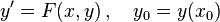
In what follows, let y be a dependent variable and x an independent variable, and y = f(x) is an unknown function of x. The notation for differentiation varies depending upon the author and upon which notation is most useful for the task at hand. In this context, the Leibniz's notation (dy/dx,d²y/dx²,...dⁿy/dxⁿ) is more useful for differentiation and integration, whereas Newton's and Lagrange's notation (y′,y′′, ... y⁽ⁿ⁾) is more useful for representing derivatives of any order compactly.

General definition of an ODE[edit]

Given F, a function of x, y, and derivatives of y. Then an equation of the form

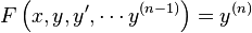
is called an explicit ordinary differential equation of order n.^[6][7]

More generally, an implicit ordinary differential equation of order n takes the form:^[8]

There are further classifications:

Autonomous

A differential equation not depending on x is called autonomous.

Linear

A differential equation is said to be linear if F can be written as a linear combination of the derivatives of y:

where a_i(x) and r(x) are continuous functions in x.^[6][9][10] Non-linear equations cannot be written in this form. The function r(x) is called thesource term, leading to two further important classifications:^[9][11]

Homogeneous: If r(x) = 0, and consequently one "automatic" solution is the trivial solution, y = 0. The solution of a linear homogeneous equation is a complementary function, denoted here by y_c.

Nonhomogeneous (or inhomogeneous): If r(x) ≠ 0. The additional solution to the complementary function is the particular integral, denoted here by y_p.

The general solution to a linear equation can be written as y = y_c + y_p.

System of ODEs[edit]

A number of coupled differential equations form a system of equations. If y is a vector whose elements are functions; y(x) = [y₁(x), y₂(x),...,y_m(x)], and F is a vector-valued function of y and its derivatives, then

is an explicit system of ordinary differential equations of order or dimension m. In column vector form:

These are not necessarily linear. The implicit analogue is:

where 0 = (0, 0,... 0) is the zero vector. In matrix form

For a system of the form , some sources also require that the Jacobian matrix be non-singular in order to call this an implicit ODE [system]; an implicit ODE system satisfying this Jacobian non-singularity condition can be transformed into an explicit ODE system. In the same sources, implicit ODE systems with a singular Jacobian are termed differential algebraic equations (DAEs). This distinction is not merely one of terminology; DAEs have fundamentally different characteristics and are generally more involved to solve than (nonsigular) ODE systems.^[12][13] Presumably for additional derivatives, the Hessian matrix and so forth are also assumed non-singular according to this scheme,^{[citation needed]} although note that any ODE of order greater than one can be [and usually is] rewritten as system of ODEs of first order,^[14] which makes the Jacobian singularity criterion sufficient for this taxonomy to be comprehensive at all orders.

Solutions[edit]

Given a differential equation

a function u: I ⊂ R → R is called the solution or integral curve for F, if u is n-times differentiable on I, and

Given two solutions u: J ⊂ R → R and v: I ⊂ R → R, u is called an extension of v if I ⊂ J and

A solution that has no extension is called a maximal solution. A solution defined on all of R is called a global solution.

A general solution of an nth-order equation is a solution containing n arbitrary independent constants of integration. A particular solution is derived from the general solution by setting the constants to particular values, often chosen to fulfill set 'initial conditions or boundary conditions'.^[15] A singular solution is a solution that cannot be obtained by assigning definite values to the arbitrary constants in the general solution.^[16]

Theories of ODEs[edit]

Singular solutions[edit]

The theory of singular solutions of ordinary and partial differential equations was a subject of research from the time of Leibniz, but only since the middle of the nineteenth century did it receive special attention. A valuable but little-known work on the subject is that of Houtain (1854).Darboux (starting in 1873) was a leader in the theory, and in the geometric interpretation of these solutions he opened a field worked by various writers, notable ones being Casorati and Cayley. To the latter is due (1872) the theory of singular solutions of differential equations of the first order as accepted circa 1900.

Reduction to quadratures[edit]

The primitive attempt in dealing with differential equations had in view a reduction to quadratures. As it had been the hope of eighteenth-century algebraists to find a method for solving the general equation of the nth degree, so it was the hope of analysts to find a general method for integrating any differential equation. Gauss (1799) showed, however, that the differential equation meets its limitations very soon unlesscomplex numbers are introduced. Hence, analysts began to substitute the study of functions, thus opening a new and fertile field. Cauchy was the first to appreciate the importance of this view. Thereafter, the real question was to be not whether a solution is possible by means of known functions or their integrals but whether a given differential equation suffices for the definition of a function of the independent variable or variables, and, if so, what are the characteristic properties of this function.

Fuchsian theory[edit]

Two memoirs by Fuchs (Crelle, 1866, 1868), inspired a novel approach, subsequently elaborated by Thomé and Frobenius. Collet was a prominent contributor beginning in 1869, although his method for integrating a non-linear system was communicated to Bertrand in 1868.Clebsch (1873) attacked the theory along lines parallel to those followed in his theory of Abelian integrals. As the latter can be classified according to the properties of the fundamental curve that remains unchanged under a rational transformation, so Clebsch proposed to classify the transcendent functions defined by the differential equations according to the invariant properties of the corresponding surfaces f = 0 under rational one-to-one transformations.

Lie's theory[edit]

From 1870, Sophus Lie's work put the theory of differential equations on a more satisfactory foundation. He showed that the integration theories of the older mathematicians can, by the introduction of what are now called Lie groups, be referred to a common source, and that ordinary differential equations that admit the same infinitesimal transformations present comparable difficulties of integration. He also emphasized the subject of transformations of contact.

Lie's group theory of differential equations has been certified, namely: (1) that it unifies the many ad hoc methods known for solving differential equations, and (2) that it provides powerful new ways to find solutions. The theory has applications to both ordinary and partial differential equations.^[17]

A general approach to solve DEs uses the symmetry property of differential equations, the continuous infinitesimal transformations of solutions to solutions (Lie theory). Continuous group theory, Lie algebras, and differential geometry are used to understand the structure of linear and nonlinear (partial) differential equations for generating integrable equations, to find its Lax pairs, recursion operators, Bäcklund transform, and finally finding exact analytic solutions to the DE.

Symmetry methods have been recognized to study differential equations, arising in mathematics, physics, engineering, and many other disciplines.

Sturm–Liouville theory[edit]

Sturm–Liouville theory is a theory of a special type of second order Ordinary Differential Equations. Their solutions are based on eigenvalues and corresponding eigenfunctions of linear operators defined in terms of second-order homogeneous linear equations. The problems are identified as Sturm-Liouville Problems (SLP) and are named after J.C.F. Sturm and J. Liouville, who studied such problems in the mid-1800s. The interesting fact about regular SLPs is that they have an infinite number of eigenvalues, and the corresponding eigenfunctions form a complete, orthogonal set, which makes orthogonal expansions possible. This is a key idea in applied mathematics, physics, and engineering. ^[18]SLPs are also useful in the analysis of certain partial differential equations.

Existence and uniqueness of solutions[edit]

There are several theorems that establish existence and uniqueness of solutions to initial value problems involving ODEs both locally and globally. The two main theorems are

Theorem	Assumption	Conclusion
Peano existence theorem	F continuous	local existence only
Picard–Lindelöf theorem	F Lipschitz continuous	local existence and uniqueness

which are both local results.

Note that uniqueness theorems like the Lipschitz one above do not apply to DAE systems, which may have multiple solutions stemming from their (non-linear) algebraic part alone.^[19]

Local existence and uniqueness theorem simplified[edit]

The theorem can be stated simply as follows.^[20] For the equation and initial value problem:

if F and ∂F/∂y are continuous in a closed rectangle

in the x-y plane, where a and b are real (symbolically: a, b ∈ ℝ) and × denotes the cartesian product, square brackets denote closed intervals, then there is an interval

for some h ∈ ℝ where the solution to the above equation and initial value problem can be found. That is, there is a solution and it is unique. Since there is no restriction on F to be linear, this applies to non-linear equations that take the form F(x, y), and it can also be applied to systems of equations.

Global uniqueness and maximum domain of solution[edit]

When the hypotheses of the Picard–Lindelöf theorem are satisfied, then local existence and uniqueness can be extended to a global result. More precisely:^[21]

For each initial condition (x₀, y₀) there exists a unique maximum (possibly infinite) open interval

such that any solution that satisfies this initial condition is a restriction of the solution that satisfies this initial condition with domain I_max.

In the case that , there are exactly two possibilities

• explosion in finite time:
• leaves domain of definition:

where Ω is the open set in which F is defined, and is its boundary.

Note that the maximum domain of the solution

• is always an interval (to have uniqueness)
• may be smaller than ℝ
• may depend on the specific choice of (x₀, y₀).

Example

This means that F(x, y) = y², which is C¹ and therefore locally Lipschitz continuous, satisfying the Picard–Lindelöf theorem.

Even in such a simple setting, the maximum domain of solution cannot be all ℝ, since the solution is

which has maximum domain:

0 \\ (x_0+\frac{1}{y_0},+\infty) & y_0

This shows clearly that the maximum interval may depend on the initial conditions. The domain of y could be taken as being , but this would lead to a domain that is not an interval, so that the side opposite to the initial condition would be disconnected from the initial condition, and therefore not uniquely determined by it.

The maximum domain is not ℝ because

which is one of the two possible cases according to the above theorem.

Reduction of order[edit]

Differential equations can usually be solved more easily if the order of the equation can be reduced.

Reduction to a first-order system[edit]

Any differential equation of order n,

can be written as a system of n first-order differential equations by defining a new family of unknown functions

for i = 1, 2,... n. The n-dimensional system of first-order coupled differential equations is then

more compactly in vector